Reaction-Diffusion Textures

Orion Sky Lawlor
2003/3/17
CS 497yyz MP1

Introduction

Reaction-diffusion textures come from a set of coupled partial differential equations that result in appealingly cellular, organic solutions.

Turk[Turk1991] quotes these as Turing's original [Turing1952], discrete 1D reaction-diffusion equations, which relate the concentrations of two chemical species $a$ and $b$, discretized into cells $a_i$ and $b_i$.

$$\Delta a_i = D_s(16-a_i b_i)+D_a (a_{i+1}-2a_i+a_{i-1})$$

$$\Delta b_i = D_s(a_i b_i-b_i-\beta_i)+D_b (b_{i+1}-2b_i+b_{i-1})$$

Here $D_s$ is the reaction rate parameter, $D_a$ and $D_b$ are diffusion rate parameters, and $\beta_i$ is a decay parameter for $b$. We can interpret $a$ as a chemical, generated in barren regions, that is consumed to produce chemical $b$. $b$ naturally decays, with an even higher decay rate where the concentration of $b$ is large. Both species diffuse, but $a$ normally diffuses faster than $b$.

Turk recommends $\beta$ of approximately 12, but picks a random slightly different value for each cell. We note nicely random results can be obtained even with fixed parameters by randomly varying the initial conditions--we found favorable results using initial values for $a$ and $b$ randomly distributed on the interval $[0,8]$. Turk recommends a diffusion rate of $D_a=0.25$ (the reaction-free stability limit) and $D_b=0.0625$. We find these parameters work well.

We note that the equation for $a$ is unstable if $b$ is negative. Since negative results can occur because of the fixed decay factor, $b$ must be clamped to zero or the solution grows without bound.

Continuous Equations

We can easily derive the multidimensional and continuous--in both space and time--version of Turing's reaction/diffusion equation. Note that we have generalized the fixed $a$ growth constant 16 to $\alpha$.

$$\frac{\partial a}{\partial t} = C_s(\alpha-a b)+C_a \nabla^2 a$$

$$\frac{\partial b}{\partial t} = C_s(a b-b-\beta)+C_b \nabla^2 b$$

Here $C_s$ is the reaction rate parameter, $C_a$ and $C_b$ are diffusion rate parameters, $\alpha$ is a growth parameter and $\beta$ is a decay parameter. We always use the values $C_s=1$, $C_a=25$, and $C_b=\frac{1}{4} C_a$, since these values result in spatial features that are a few units across.

In practice, we must (re)discretize this continuous set of equations in both space and time in order to solve this system. Using the first-order Euler method, this recovers Turing's original discrete equations--that is, these continuous equations can be seen as a way to derive consistent parameters for the discrete equations. For a timestep of $\Delta t$, $D_s = C_s \Delta t$. For a uniform mesh size $h$, in 2D $D_a = C_a \frac{\Delta t}{h^2}$ and similarly $D_b = C_b \frac{\Delta t}{h^2}$. We of course always choose $\Delta t$ as large as possible--the theoretical diffusion stability criterion requires $D_a \le 0.25$; and the nonlinear reaction rate also has some limit, which appears to be near $D_s \le 0.05$.

Multigrid

The advantage of using a continuous formulation is that we can take advantage of the powerful tools available for quickly solving partial differential equations, such as the multigrid method. For small grid spacings and large domains, multigrid can dramatically accellerate convergence, as illustrated in Figure 1. We find the coarse-to-fine direction of multigrid to be sufficient--no reverse restriction is required.

No multigrid, after 1,000 steps.	No multigrid, after 50,000 steps.
No multigrid, after 350,000 steps.	Multigrid, after 1,000 steps.

Figure 1. Illustrating the dramatic speed advantages of multigrid on a 1024x1024 domain with a grid spacing of $h=1/8$. $a$ concentration is shown in red; $b$ is shown in green.

Parameters

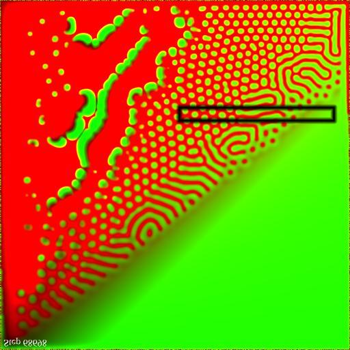
The character of the solutions to this equation depends strongly on the ratio $\alpha/\beta$, as illustrated in the parameter map below. Interesting, spatially varying results only appear for $\alpha/\beta$ near one. Larger values over-active, which results in $b$ dominating; while smaller values fail to achieve a self-sustaining quantity of $b$, which results in unstable pulsating patterns. In the remainder, we fix $\beta$ at 20 and vary the growth rate $\alpha$ between 17.5 and 27.5, as shown in the dark box.

Figure 2.Parameter map for growth and decay parameters. The growth rate $\alpha$ varies along the X axis from 0 at the left edge to 30 at the right edge. The decay rate $\beta$ varies along the Y axis from 0 at the bottom edge to 30 at the top.

Growth Parameter Variation

Grayscale version of growth coefficient.

Resulting output texture.

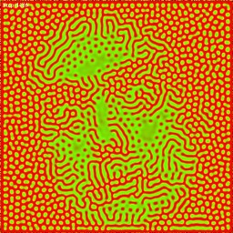
Figure 3.Varying growth parameter according to a photograph for a bizarre effect.

Growth Parameter Variation

We applied this reaction-diffusion texture generation method to a global illumination raytracer-like renderer developed by the author (the method is similar to a conetracer [Lawlor1999]).

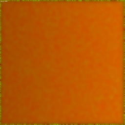
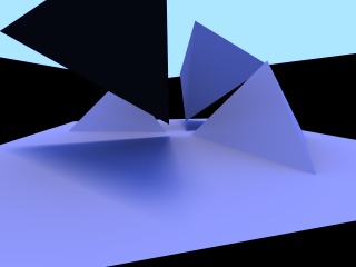Globally illuminated scene without texture.

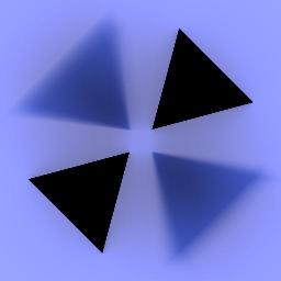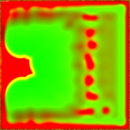
Illumination on ground plane.	Growth rate derived from illumination.
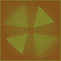
Grown texture.	Grown texture, recolored.

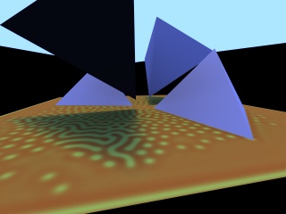(900K MPEG Movie, 320x240)
Scene rendered using grown texture.

References

• [Lawlor1999] Orion Lawlor, Conetracer Project Page, http://charm.cs.uiuc.edu/users/olawlor/projects/1999/conetracer/index.html.
• [Turk1991] Greg Turk, "Generating Textures on Arbitrary Surfaces Using Reaction-Diffusion," Computer Graphics, Vol. 25, No. 4, (SIGGRAPH 91), July 1991, pp. 289-298.
• [Turing1952] Alan Turing, "The Chemical Basis of Morphogenesis," Philosophical Transactions of the Royal Society B, Vol. 237, pp. 37-72 (August 14, 1952).

Back to Orion's Oeuvre.
Back to Orion's Home Page.